How to run the Test Suite
The Test Suite is a set of examples of fits, which are useful to
learn the peculiarities of the program by actually doing fits.
Another important use of the Suite is to check that the algorithm is
fully functional in your particular CASA installation. The results of
all the fits (performed in a machine where UVMultiFit is fully
functional) can be seen in the directory called ALLFITS.RESULTS,
so that the user can compare his/her results with these.
To run the Suite, just follow these steps:
1 Edit the script called TEST_ALL.py, so that it fits your needs and the particularities of your system. The parameters to be set are:
DoSimObs(a boolean; default True). Re-generate all the simulated datasets (this step is only needed for the first time that you run the Test Suite)DoFit(a boolean; default True). Re-do all the example fits.casaexe(a string; defaultcasa --nologger). Execution command for CASA (avoinding the logger; the exact command may depend on your installation).
2 Execute CASA from the directory of the Test Suite.
3 From the CASA prompt, execute the master script:
>>> execfile('TEST_ALL.py')
The script will create several diagnostic files in two directories:
FIT_SCRIPTS: all the scripts used in the fits (with the model definitions, initial parameters, bounds, etc.). These scripts are automatically generated.ALLTESTS.RESULTS: Plots of dirty images, post-fit residual images, parameter plots (for spectral-line fits), and the filefit_results.dat.
In the file fit_results.dat, located in the ALLTESTS.RESULTS
directory, the user will find the fitted parameter values,
together with the true values used in the simulations and the
execution times for all fittings.
If you want to run one particular test, go to its directory (‘TEST*’)
and execute the script named MASTER*.py. Notice that you will need
to define the DoSimobs, DoFit and casaexe parameters manually,
within the CASA session, before running the script.
The MASTER*.py script in each TEST directory generates the simulated
data and creates the fitting scripts, which are then executed in independent
casa sessions, through calls with os.system.
The fitting scripts created by MASTER*.py are based on the templates
called test*.py, which are located in the same TEST directory. If you
want to change any detail in the simulation and/or fitting strategy used
in the tests, you may need to change both, the MASTER*.py and the
test*.py scripts.
Description of the Tests
TEST 1 Fitting a source ellipticity. the source appears unresolved in the image plane. The axis ratio and position angle estimated by the algorithm are, within uncertainties, compatible with the ones used in the simulation. The code used is:
>>> visname = 'Disc/Disc.alma.out10.noisy.ms'
>>> modelshape = 'disc'
>>> modvars = '0,0,p[0]*(nu/5.e+10)**p[1],p[2],p[3],p[4]'
>>> pini = [0.8, 0., 0.24, 0.4, 45.]
>>> parbound = [[0., None],[-2.,2.],[0.,None],[0.1,0.9],[0.,180.]]
>>>
>>> myfit = uvm.uvmultifit(vis = visname, spw = '0',
>>>             model = modelshape, OneFitPerChannel = False,
>>>             var = modvars,write='residuals',
>>>             p_ini = pini,
>>>             bounds=parbound)
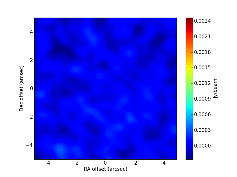
The simulated parameter values are:
[0.244, 1., 0.2, 0.5, 60.]. The CLEAN image (left) and that of the post-fit residuals (right) are: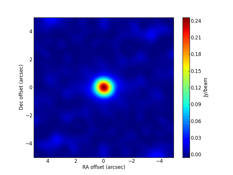
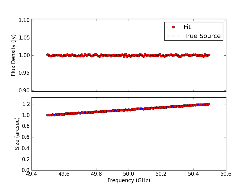
TEST 2 Fitting sources with different radial intensity profiles. All sources appear unresolved in the image plane, but the source sizes are fitted with remarkable precision in Fourier space. The post-fit residuals are all very low, with the exception of the
power-2source.Note
Take into account that the
power-2source has an infinite flux density, since the source extends to infinity and its 2-dimensional integral does not converge. Hence, the shortest baselines (i.e. the ones corresponding to the spatial scales of the order of the image size used in the simulation) have to be removed before the fitting (they are biased toward lower flux densities).Furthermore, this window effect from the image used by simobserve introduces artifacts in the residual image, though such bad residuals are not indicative of a wrong fit; these are due to the fact that
simobservehas not used an exactpower-2model for the simulation (the model image is a truncated representation of the source).A similar thing happens with the fit to the
expomodel, which also presents some post-fit residual artifacts (notice the hint of a missing-flux effect in the residual image).The code used in the fit to the
bubble(it is similar for the rest of profiles tested) is:>>> visname = 'bubble/bubble.alma.out10.noisy.ms' >>> modshape = 'bubble' >>> shapevar = 'p[2],p[3],p[0],p[1],1.0,0.0' >>> pi = [0.8, 1.200e+00,0.,0.] >>> parbound = [[0.,None],[0.,1.500e+00],[-1.,1.],[-1.,1.]]
>>> myfit = uvm.uvmultifit(vis = visname, write='residuals',
>>>         spw = '0', model = modshape, OneFitPerChannel = True,
>>>         var = shapevar, p_ini = pi, bounds = parbound)
The fitted size (and flux density) as a function of frequency, for the case of the Gaussian radial intensity profile is:
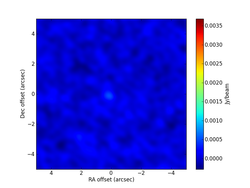
TEST 3 Fitting multiple sources simultaneously. The compound source is made of a disc with a hole (the hole is modelled using an inner disc with a negative flux density) and a Gaussian with an offset position. Notice that for the hole model to work, the surface brightness of the two discs must be the same (in absolute value). All sources appear unresolved in the image plane, but the fitted parameters are compatible, within uncertainties, with the values used in the simulation. The code used in the fit is:
>>> visname = 'Discs_Gaussian/Discs_Gaussian.alma.out10.noisy.ms'
>>> modelshape = ['disc','disc','Gaussian']
>>> modvars = ['0.,0.,p[0],p[1],1.,0.',
>>>            '0.,0.,-p[0]*p[2]**2.,p[1]*p[2],1.,0.',
>>>            '0.,p[3],p[4],p[5],1.,0.']
>>> pini = [0.17, 0.65, 0.4, -1.5, 0.6, 0.52]
>>> parbound = [[0.,None],[0.,None],[0.,None],
>>>             [-15,15],[0.,None],[0.,None]]
>>>
>>> myfit = uvm.uvmultifit(vis = visname, spw = '0',
>>>         model = modelshape, OneFitPerChannel = False,
>>>         var = modvars,write='residuals',
>>>         p_ini = pini,
>>>         bounds=parbound)
The parameter values in the simulation are:
[0.248, 0.5, 0.5, -2., 0.5, 0.4]. The CLEAN image (left) and that of the post-fit residuals (right) are: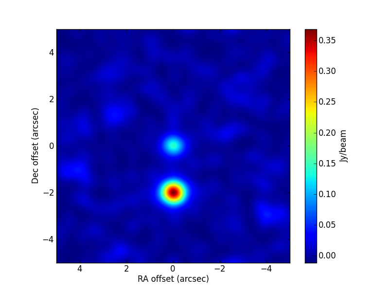
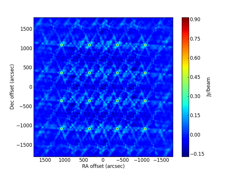
TEST 4 Widefield mosaic. Simulation of an L-band J-VLA mosaic with three pointings, covering an area of about 1 degree squared. The sources are distributed in a grid accross the mosaic area. This dataset is useful to check the primary-beam correction and the mosaic w-projection algorithm. The code used in this fit is:
>>> msout = 'WideField/WideField.vla.d.noisy.ms'
>>> model = ['delta' for i in range(16)]
>>> modvars = ['1080.000+p[0], -1080.000+p[1], p[2]','1080.000+p[3], -360.000+p[4], p[5]',
>>>        '1080.000+p[6],  360.000+p[7], p[8]','1080.000+p[9], 1080.000+p[10], p[11]',
>>>        ' 360.000+p[12], -1080.000+p[13], p[14]',' 360.000+p[15], -360.000+p[16], p[17]',
>>>        ' 360.000+p[18],  360.000+p[19], p[20]',' 360.000+p[21], 1080.000+p[22], p[23]',
>>>        '-360.000+p[24], -1080.000+p[25], p[26]','-360.000+p[27], -360.000+p[28], p[29]',
>>>        '-360.000+p[30],  360.000+p[31], p[32]','-360.000+p[33], 1080.000+p[34], p[35]',
>>>        '-1080.000+p[36], -1080.000+p[37], p[38]','-1080.000+p[39], -360.000+p[40], p[41]',
>>>        '-1080.000+p[42],  360.000+p[43], p[44]','-1080.000+p[45], 1080.000+p[46], p[47]']
>>> pini = [0.0 for i in range(48)]
>>> pini[::3] = 0.8  # Initial estimates of flux densities. You can change this to crazy
>>>                  # values, is you like.
>>> phref = 'J2000 10h00m00.08s 30d00m02.0s'
>>> bounds = []
>>> for i in range(16):
>>> bounds += [[-5.,5],[-5.,5.],[0.,None]]
>>> myfit = uvm.uvmultifit(vis=msout, model=model, var=modvars, field=field,
>>>     p_ini=pini, NCPU = 4, column='data',write='residuals',
>>>     OneFitPerChannel=False, phase_center=phref,pbeam=True,
>>>     dish_diameter=25.0, ldfac = 1.0, LMtune=[1.e-3,10.,1.e-5,10],bounds=bounds)
All sources have a flux density of 1 Jy in the simulation. The CLEAN image (left, computed with W projection) and that of the post-fit residuals (right) are:
TEST 5 A Gaussian source observed with Plateau de Bure. A time-varying gain amplitude is added to one of the antennas. We use the gain solver feature, to solve for the source parameters and the antenna gain simultaneously, approximating the gain with a
piece-wisetime-evolving function.Note
The gain-solver feature is experimental. In realistic situations, a lot of fitting parameters may be needed, to solve for all the antenna gains with enough time resolution, although this method should be superior to the conventional selfcal scheme, where the gaincal has no memory of the gain values that are close by in time.
The code used in this fit is:
>>> LMtune = [1.e-5,10.,1.e-5,10]
>>> visname = 'Gaussian/Gaussian.pdbi-a.noisy.ms'
>>> amp_gains = {2:'pieceWise(p[4],p[5],0.0,1795.)'}
>>> modelshape = ['Gaussian']
>>> modvars = ['0.,0.,p[0],p[1],p[2],p[3]']
>>> pini = [2.45, 1.95, 0.53, 33., 0.8, 1.2]
>>> parbound = [[0.,None],[0.,None],[0.,None],[0.,90.],[0.75,1.25],[1.1,1.9]]
>>> myfit = uvm.uvmultifit(vis = visname, spw = '0',
>>>          model = modelshape, OneFitPerChannel = False,
>>>          var = modvars, write = 'residuals',LMtune=LMtune,
>>>          p_ini = pini, amp_gains = amp_gains,
>>>          bounds=parbound)
That is, the gain is modelled by parameters
p[4]andp[5](i.e., initial and final gain, assuming a linear change from the start of the observations until 1795 seconds afterwards (i.e., the end of the observations). The simulated values are[3.5, 1.5, 0.667, 45., 1., 1.5]. The CLEAN image (left, with no selfcal applied) and that of the post-fit residuals (right) are: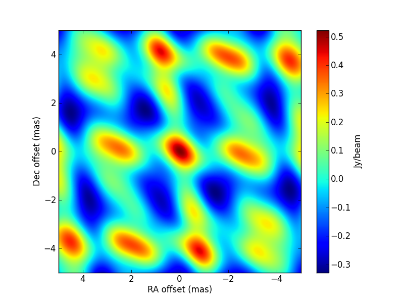
TEST 6 Test of
immultifit. A simple model (two Gaussians) is fitted to the gridded visibilities in the image plane. The code used is:>>> immname = 'TEST6.CLEAN.residual' >>> psfname = 'TEST6.CLEAN.psf' >>> modelshape = ['Gaussian','Gaussian'] >>> modvars = ['0.,0.,p[0],p[1],1.,0.', '0.,p[2],p[3],p[4],1.,0.'] >>> pini = [0.7, 0.26, -1.13, 0.6, 0.52] >>> parbound = [[0.,None],[0.,None],[-15,15],[0.,None],[0.,None]] >>> >>> myfit = uvm.immultifit(residual = immname, psf = psfname, >>> model = modelshape, OneFitPerChannel = False, >>> var = modvars,write='residuals', >>> p_ini = pini,LMtune=[1.e-3,10.,1.e-8,200,1.e-5], >>> bounds=parbound)
The parameter values used in the simulation are
[1., 0.2, -1.5, 0.5, 0.4]. The best-fit image is: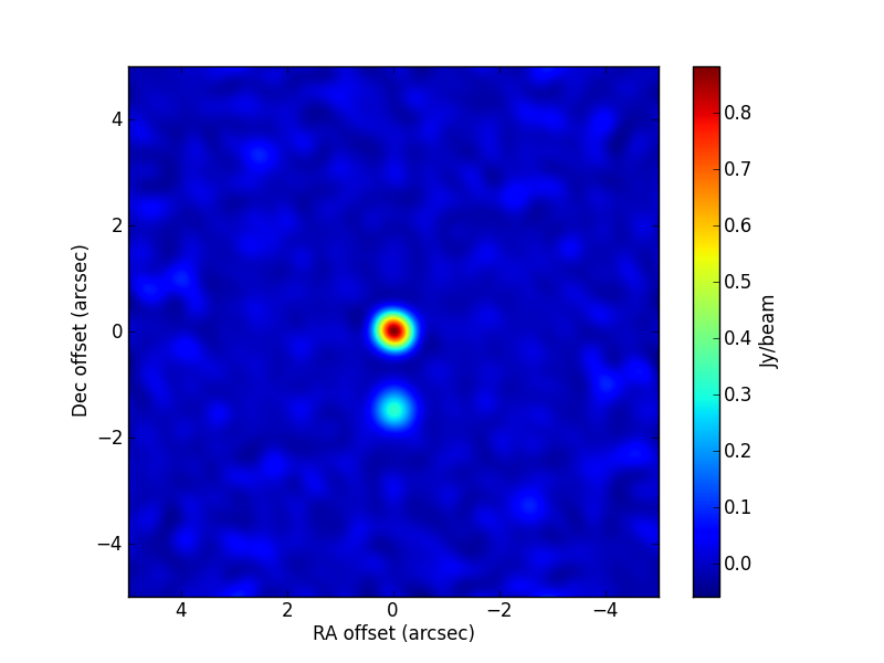
TEST 7 A test of the
only_fluxfitting mode, which can be used to fit many (tens or even hundreds!) source components whose shapes and coordinates are fixed in the model (i.e., only the flux densities are fitted).Note
This mode can be used as an interface to implement modelling based on compressed-sensing techniques. The user can also load CLEAN models and fit for the flux-densities of each delta component (say, for instance, at different scans, to check for structure variability, as it was done in Marti-Vidal et al. 2016, A&A, 593, A61; Sect. 3.1.2).
The code used in the test is:
>>> visname = 'Only_Flux/Only_Flux.alma.out10.noisy.ms'
>>> modelshape = ['disc', 'disc', 'Gaussian', 'Gaussian', 'Gaussian', 'disc']
>>>
>>> modvars = ['0., 0., p[0], 0.5, 1., 0.', '2., 0., p[1], 0.25, 1., 0.',
>>>            '0., -2., p[2], 0.4, 1., 0.', '-4., 0., p[3], 0.1, 1., 0.',
>>>            '-2., 2., p[4], 0.4, 1., 0.', '-4., -2., p[5], 0.85, 1., 0.']
>>>
>>> pini = [1.486e-01,2.972e-01,4.500e-01,5.000e-01,1.200e+00,4.459e-02]
>>>
>>> parbound = None # Let's be wild!
>>> myfit = uvm.uvmultifit(vis = visname, spw = '0',
>>>          model = modelshape, OneFitPerChannel = False,
>>>          var = modvars, write='residuals',
>>>          p_ini = pini, only_flux=True,
>>>          bounds=parbound)
The parameter values used in the simulation are:
[0.2477,0.1858,0.25,2.5,1.5,0.03716]. The CLEAN image (left) and that of the post-fit residuals (right) are: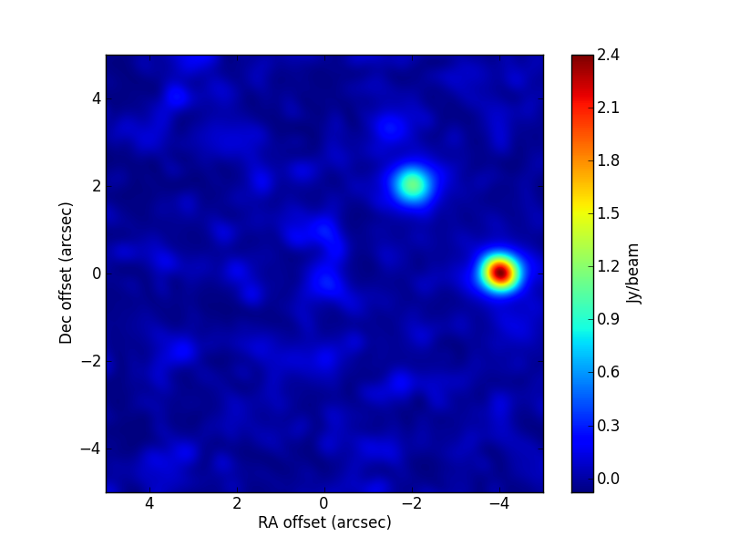

Note
Notice that, in this test,
simobserveintroduces a small sub-pixel shift in RA, which introduces small systematic residuals when the sources are fixed to their nominal simulated positions (look at the plot of residuals). This effect would disappear if the position was fitted prior to the only-flux fit.
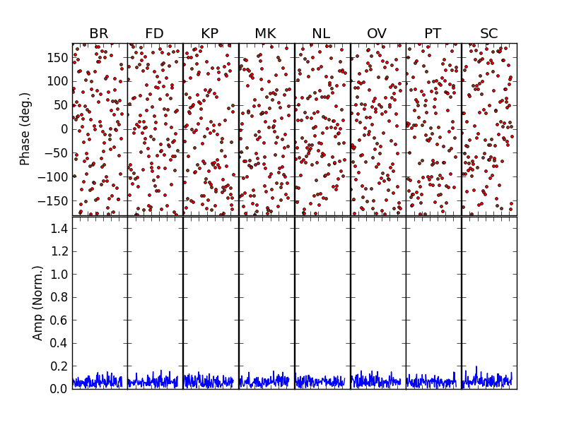
TEST 8 An example of global fringe fitting (GFF), a-la UVMultiFit. A synthetic C-band VLBA dataset is generated with realistic noise and 128 channels (covering 32 MHz). the gains are estimated first by fitting them to the peaks in delay-rate space (using the new helper rutine “QuinnFF”). These estimates are then used as a-priori values for the least-squares GFF modeling.
Note
Notice that GFF calibration tables are not generated by UVMultiFit (that feature is beyond the purpose of the program, at least in its current version), but the calibrated data can still be generated by dividing the data by the (gain-corrected) model (which UVMultiFit writes in the model column, when you set
write='model'). The master script in the test directory shows how to do this.You can also save the calibrated data with
write='calibrated'(in the next release of the code).A fixed point source is used for the GFF (centered at the nominal source position), but (of course) more complicated structures (and even CASA
*.modelimages generated with clean/tclean) can be used as models… and you can even fit them together with the gains!The most important part of the script (i.e., where the gain models are defined) are:
>>> REFANT = 'LA'
>>>
>>> # Get the names of the antennas:
>>> tb.open('VLBA_GFF.noisy.ms/ANTENNA')
>>> ANTNAMES = list(tb.getcol('NAME'))
>>> tb.close()
>>>
>>> allgains = {}
>>>
>>> # Set the gain models (the REFANT will have a null phase gain):
>>>
>>> ai = 0 # Number of antennas with gains already set.
>>>
>>> for ant in range(len(ANTNAMES)):
>>>
>>>    pc = 3*ai # Current parameter number
>>>
>>>    if ANTNAMES[ant] != REFANT:
>>>       allgains[ant] = '6.2832*(p[%i]*(nu - nu0)*(1.e-9) + p[%i]*t) + p[%i]'%(pc,pc+1,pc+2)
>>>       ai += 1
>>> # i.e., for each antenna, the gain parameters are ordered by delay, rate, and phase.
>>>
>>> # Total number of fitting parameters:
>>> Npar = len(allgains.keys())*3
>>>
>>> # Create instance (but don't fit yet). Notice that the source model
>>> # is a delta component with fixed coordinates and flux (set to 1 Jy).
>>>
>>> myfit = uvm.uvmultifit(vis='VLBA_GFF.noisy.ms', spw='0', column='data',
>>>            scans = [0], stokes = 'RR', model = ['delta'], var=['0,0,1'],
>>>            write='model',NCPU=4, p_ini=[0.0 for i in range(Npar)],
>>>            OneFitPerChannel=False, finetune=True,
>>>            phase_gains = allgains, LMtune=[1.e-3,10.,1.e-4,5,1.e-3])
>>>
>>> Get gain estimates from the helper GFF function:
>>> QGains = myfit.QuinnFF(0, ANTNAMES.index(REFANT), 0, 1)
>>>
>>> # Set the initial parameter values from the output of QuinnFF:
>>>
>>> pini = []
>>> for ant in range(len(ANTNAMES)):
>>>    if ant != ANTNAMES.index(REFANT):
>>>       pini += [QGains[0][ant]*1.e9, QGains[1][ant], QGains[2][ant]]
>>>
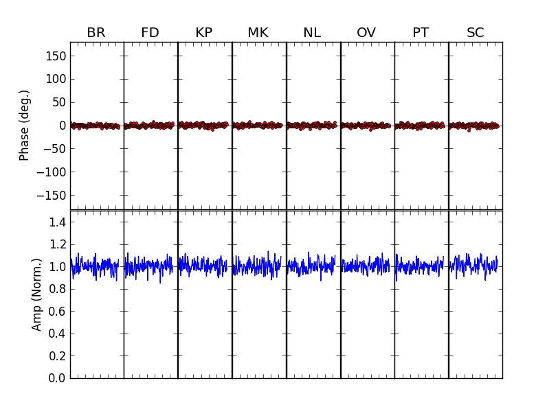
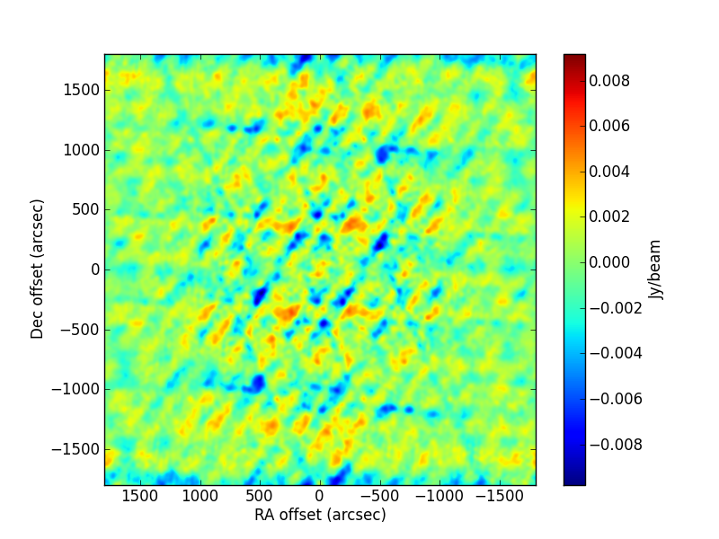
After these lines, just running
fit()would perform the GFF on the first scan of the dataset (scan 0). The user could then loop over scans (runningreadData()andinitModel()at each scan), to fringe-fit the whole dataset in the same way. The scan-averaged visibilities before (left) and after (right) the GFF calibration are: